How Fast Is PyJuice? Testing Compilation Speed Across GPUs and Batch Sizes

Table of Links

Abstract and 1. Introduction

2. Preliminaries and Related Work

3. Key Bottlenecks in PC Parallelization

4. Harnessing Block-Based PC Parallelization

   4.1. Fully Connected Sum Layers

   4.2. Generalizing To Practical Sum Layers

   4.3. Efficient Implementations by Compiling PC Layers

   4.4. Analysis: IO and Computation Overhead

5. Optimizing Backpropagation with PC Flows

6. Experiments

   6.1. Faster Models with PyJuice

   6.2. Better PCs At Scale

   6.3. Benchmarking Existing PCs

7. Conclusion, Acknowledgements, Impact Statement, and References

A. Algorithm Details

B. Additional Technical Details

C. Experimental Details

D. Additional Experiments

D. Additional Experiments

D.1. Speed of the Compilation Process

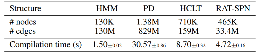
In Table 5, we show the compilation speed of PCs with different structures and different sizes. Experiments are conducted on a server with an AMD EPYC 7763 64-Core Processor and 8 RTX 4090 GPUs (we only use one GPU). The results demonstrate the efficiency of the compilation process, where even the PD model with close to 1B parameters can be compiled in around 30 seconds.

D.2. Runtime on Different GPUs

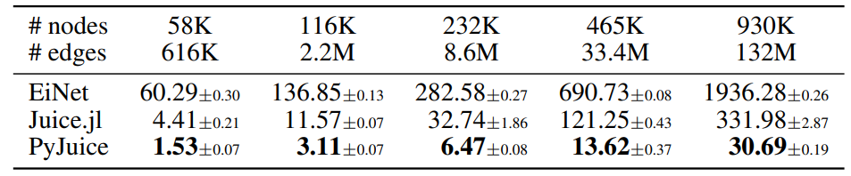
In addition to the RTX 4090 GPU adopted in the experiments in Table 1, we compare the runtime of PyJuice with the baselines on an NVIDIA A40 GPU. As shown in the following table, PyJuice is still significantly faster than all baselines for PCs of different sizes.

D.3. Runtime on Different Batch Sizes

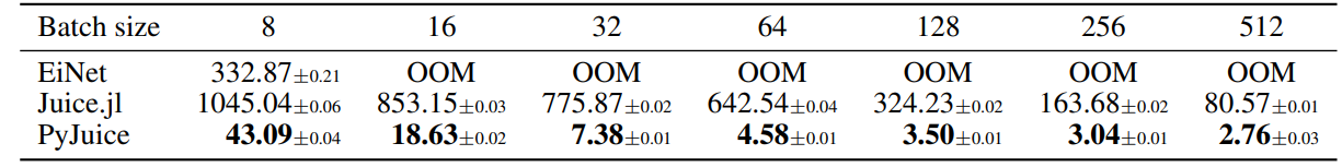
As a supplement to Table 1, we report the runtime for a RAT-SPN (Peharz et al., 2020b) with 465K nodes and 33.4M edges using batch sizes {8, 16, 32, 64, 128, 256, 512}. To minimize distractions, we only record the time to compute the forward and backward process, but not the time used for EM updates. Results are shown in the table below.